
TL;DR: We replace the hand-tuned NMS or DBSCAN step at the end of 3D keypoint detectors with a small learned graph network that decides which candidates to keep and moves them onto the correct location.
Abstract
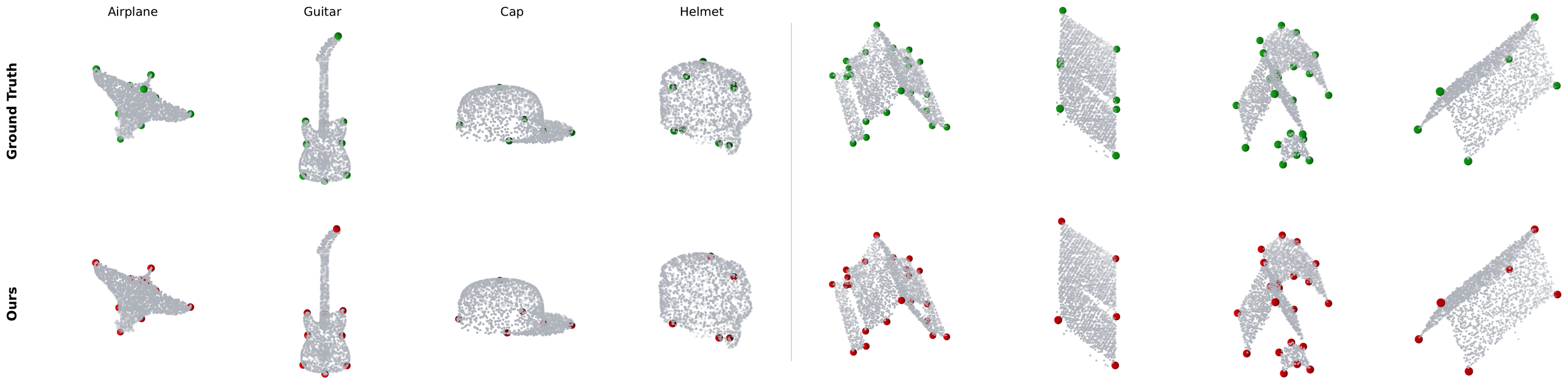
Detecting 3D keypoints is a long-standing challenge in computer vision. Most detectors end with a heuristic post-processing step that is not learned. We propose a 3D keypoint detector that improves on this step with a learned suppression module, paired with a Point Transformer backbone that we extend with a directional graph neural network. The module is a graph network over candidates that learns which to keep, which to suppress, and how to relocate the remaining ones. Paired with three backbones, it improves over DBSCAN and greedy non-maximum suppression, and because it operates on candidate features rather than raw geometry, the same formulation applies to both structural and semantic keypoints. Our model surpasses the per-category trained KeypointDETR on 12 of 16 KeypointNet categories, attains the best Corner F1 on the Building3D Entry-Level benchmark, and remains competitive with BWFormer on the larger Tallinn split.
Method
Backbone
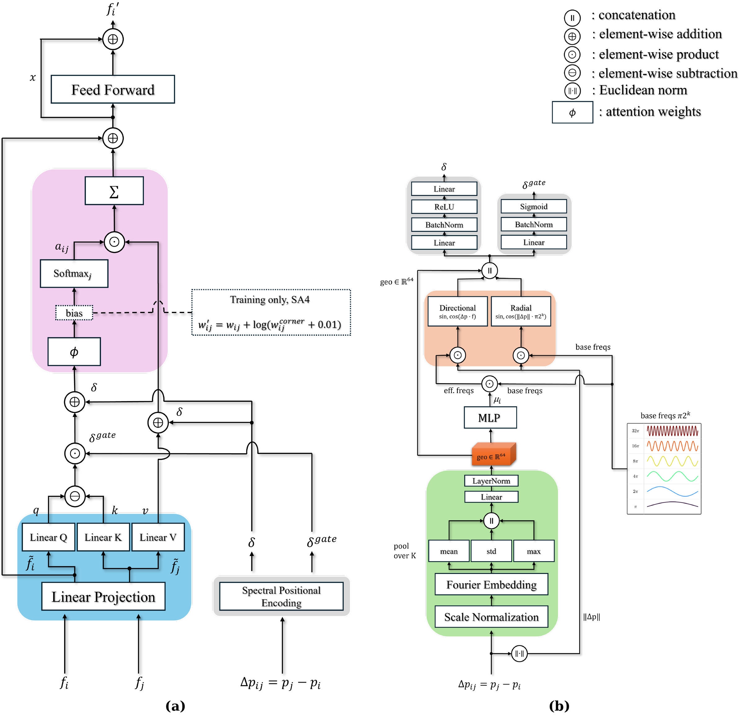
The backbone predicts, for every point, a keypoint probability and an offset to the nearest keypoint. It builds on a hierarchical Point Transformer encoder with two extensions: a spectral positional encoding that adapts its frequency bands to the geometry of each local neighborhood, and a directional graph neural network after the decoder that passes signed, direction-aware messages between neighboring points to reinforce geometrically distinctive locations such as corners.
Point Transformer block and spectral positional encoding
Learned suppression
High-confidence points vote at their offset-displaced positions, and the votes are reduced to a small candidate set. Instead of a fixed rule deciding which candidates survive, a graph network over the candidates makes that decision. In each of two message-passing rounds, every pair of nearby candidates predicts how strongly one suppresses the other, each candidate updates its state from the suppression it receives, and then moves toward a better position before the next round. A final keep score, discounted by the strongest suppression a candidate received, selects the output keypoints.
Earlier learned NMS only rescored detections in place. In 3D a keypoint rarely coincides with any candidate, so relocation is what lets the module improve localization, not just selection. The module adds 0.15M parameters and is trained on top of the frozen backbone.
- \(h_j \gets \mathrm{MLP}_{\mathrm{emb}}(z_j)\)shared embedding into \(\mathbb{R}^{128}\)
- for \(t = 1,\dots,T\) do
- \(d_{ij} \gets \lVert c_i - c_j \rVert,\;\; \mathcal{A} \gets \{(i,j): d_{ij} < \rho,\ i \neq j\}\)
- \(s_{ij} \gets \sigma\big(\mathrm{MLP}_{\mathrm{rel}}([\,h_i, h_j, d_{ij}\,])\big)\) for \((i,j)\in\mathcal{A}\), else \(0\)\(s_{ij}\): \(i\) suppresses \(j\)
- \(u_j \gets \sum_i s_{ij}\, h_i\)incoming suppression
- \(h_j \gets h_j + \mathrm{MLP}_{\mathrm{upd}}([\,h_j, u_j\,])\)
- \(c_j \gets c_j + \mathrm{MLP}_{\mathrm{mov}}(h_j)\)relocate; \(c_j\) accumulates the displacement
- end for
- \(\pi_j \gets \sigma\big(\mathrm{MLP}_{\mathrm{keep}}(h_j)\big)\cdot\big(1 - \max_i s_{ij}\big)\)\(s_{ij}\) from the final round
- return \(\{c_j : \pi_j > \tau\}\)
def learned_suppression(z, c):                                       # z: [K, D], c: [K, 3]
    h = mlp_emb(z)                                                   # 1
    for t in range(T):                                               # 2
        d = torch.cdist(c, c)                                        # 3
        A = (d < rho) & ~torch.eye(len(c), dtype=torch.bool)
        s = torch.sigmoid(mlp_rel[t](pairs(h, d)).squeeze(-1)) * A   # 4  s[i, j]: i suppresses j
        u = s.T @ h                                                  # 5  incoming suppression
        h = h + mlp_upd[t](torch.cat([h, u], dim=-1))                # 6
        c = c + mlp_mov[t](h)                                        # 7  relocate
    keep = torch.sigmoid(mlp_keep(h)).squeeze(-1)
    pi = keep * (1 - s.max(dim=0).values)                            # 9
    return c[pi > tau]                                               # 10
\(\mathrm{MLP}_{\mathrm{emb}}\) and \(\mathrm{MLP}_{\mathrm{keep}}\) are shared across rounds; \(\mathrm{MLP}_{\mathrm{rel}}\), \(\mathrm{MLP}_{\mathrm{upd}}\), and \(\mathrm{MLP}_{\mathrm{mov}}\) have independent weights in each round \(t\). \(\rho\): suppression radius; \(T\): message-passing rounds per forward pass; \(\tau\): keep threshold. pairs(h, d) builds \([\,h_i, h_j, d_{ij}\,]\) for every pair.
Results
Learned suppression versus heuristic post-processing
Swapping only the post-processing stage, on three different backbones, learned suppression gives the best Corner F1 and mIoU in every case.
| Backbone | Post-processing | Entry-Level CF1 | Tallinn CF1 | KeypointNet mIoU |
|---|---|---|---|---|
| Ours | Greedy NMS | 90.70 | 85.10 | 84.25 |
| DBSCAN | 89.00 | 83.60 | 79.67 | |
| Learned suppression | 93.20 | 87.80 | 92.01 | |
| PointNet++ | Greedy NMS | 60.40 | 68.30 | 46.33 |
| DBSCAN | 82.30 | 80.40 | 70.92 | |
| Learned suppression | 87.00 | 84.90 | 74.99 | |
| DGCNN | Greedy NMS | 43.00 | 44.30 | 42.87 |
| DBSCAN | 78.40 | 74.90 | 70.68 | |
| Learned suppression | 84.90 | 81.70 | 77.87 |
Compare the three post-processing methods in 3D at the top of the page.
Building3D: roof corners from airborne LiDAR
Our detector reaches the best Corner Recall and F1 on Entry-Level and stays competitive with BWFormer on the full Tallinn split, without the roof-specific priors used by PBWR and BWFormer.
| Method | ACO↓ | CP | CR | CF1 |
|---|---|---|---|---|
| Supervised (PT) | 0.26 | 89.0 | 66.0 | 76.0 |
| PBWR | 0.22 | 97.0 | 85.0 | 91.0 |
| Ours | 0.22 | 96.5 | 90.1 | 93.2 |
| Method | ACO↓ | CP | CR | CF1 |
|---|---|---|---|---|
| PBWR | 0.222 | 98.5 | 68.8 | 81.0 |
| BWFormer | 0.204 | 94.9 | 82.7 | 88.4 |
| Ours | 0.216 | 92.3 | 83.7 | 87.8 |
Selected rows; the paper reports the full comparison with prior methods.

KeypointNet: semantic landmarks across 16 categories
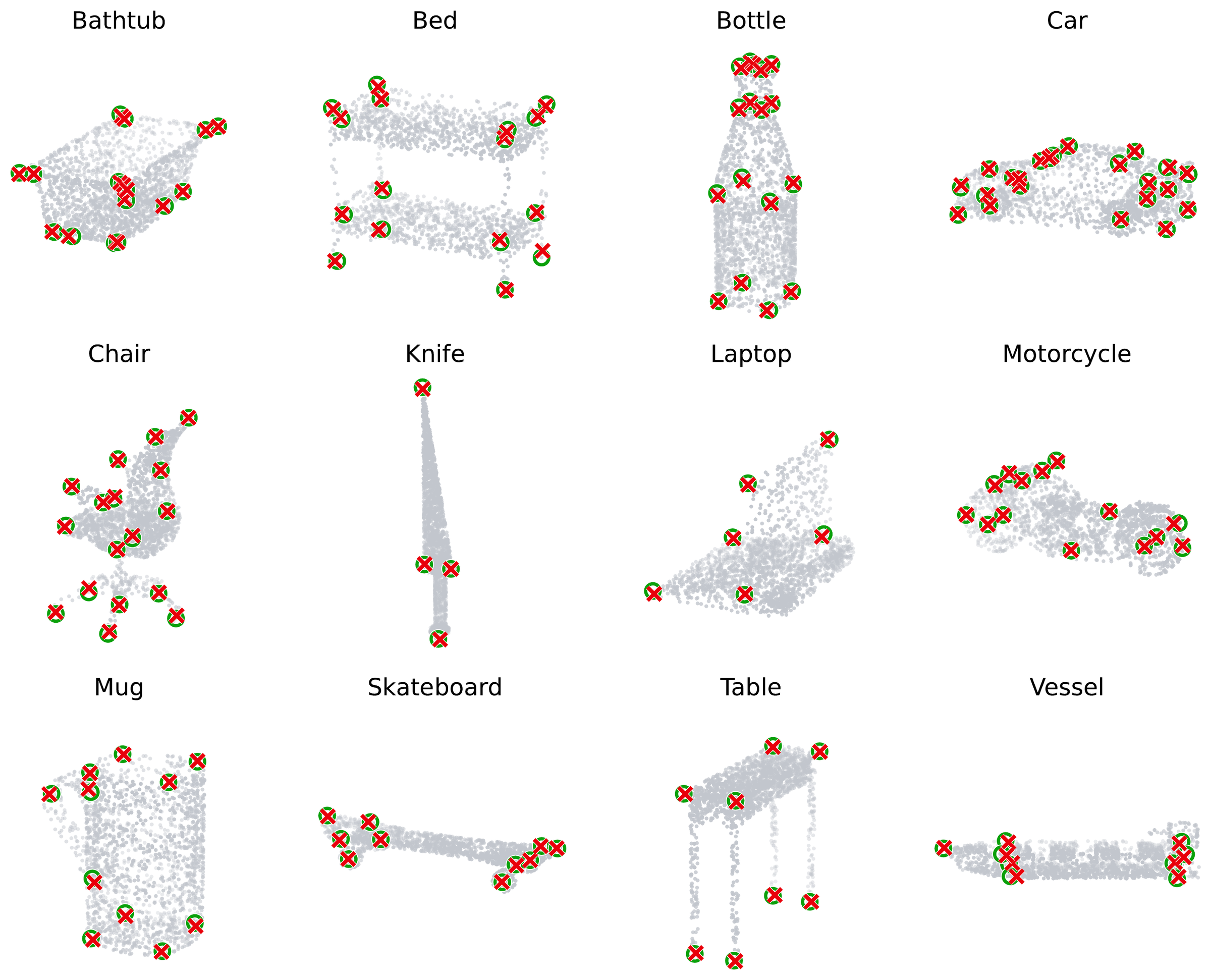
A single model trained on all 16 categories surpasses KeypointDETR on 12 of them. KeypointDETR is trained per category with a fixed keypoint set per category, so the two methods are trained under different regimes; this comparison is best read as a single cross-category model against per-category specialists.
Per-category numbers, with Chamfer distance
| Category | KeypointDETR mIoU | Ours mIoU | KeypointDETR CD↓ | Ours CD↓ |
|---|---|---|---|---|
| Airplane | 91.37 | 96.93 | 0.045 | 0.038 |
| Bathtub | 71.37 | 90.83 | 0.074 | 0.049 |
| Bed | 70.83 | 87.61 | 0.081 | 0.056 |
| Bottle | 87.22 | 90.68 | 0.050 | 0.049 |
| Cap | 79.43 | 91.74 | 0.066 | 0.062 |
| Car | 94.29 | 92.25 | 0.045 | 0.051 |
| Chair | 91.89 | 94.58 | 0.055 | 0.051 |
| Guitar | 93.96 | 97.84 | 0.045 | 0.029 |
| Helmet | 85.05 | 52.36 | 0.087 | 0.407 |
| Knife | 63.12 | 91.12 | 0.089 | 0.036 |
| Laptop | 99.11 | 99.65 | 0.024 | 0.033 |
| Motorcycle | 87.52 | 92.28 | 0.053 | 0.047 |
| Mug | 96.62 | 85.55 | 0.049 | 0.096 |
| Skateboard | 92.28 | 94.25 | 0.055 | 0.037 |
| Table | 98.05 | 95.96 | 0.027 | 0.059 |
| Vessel | 59.97 | 77.35 | 0.105 | 0.079 |
Where it fails. Helmet is our weakest category. The detector relies on locally distinctive geometry and has no category template, while Helmet's landmarks are semantic conventions on a smooth shell. Cap has a similarly smooth overall shape, but its landmarks sit on the sharp brim, and the same model reaches 91.74 mIoU there.
BibTeX
@misc{bekar2026learnedsuppression3dkeypoint,
title={Learned Suppression for 3D Keypoint Detection with a Graph-Transformer Backbone},
author={Batuhan Arda Bekar and Can Sarı and Hüseyin Can Gülkan and Barış Özcan},
year={2026},
eprint={2605.15088},
archivePrefix={arXiv},
primaryClass={cs.CV},
url={https://arxiv.org/abs/2605.15088},
}